General project setup
We setup a project using a hexagonal canvas with a cell size of 500 km. The project is set in-memory but for a real case study you would like to set path to a persistent location on disk.
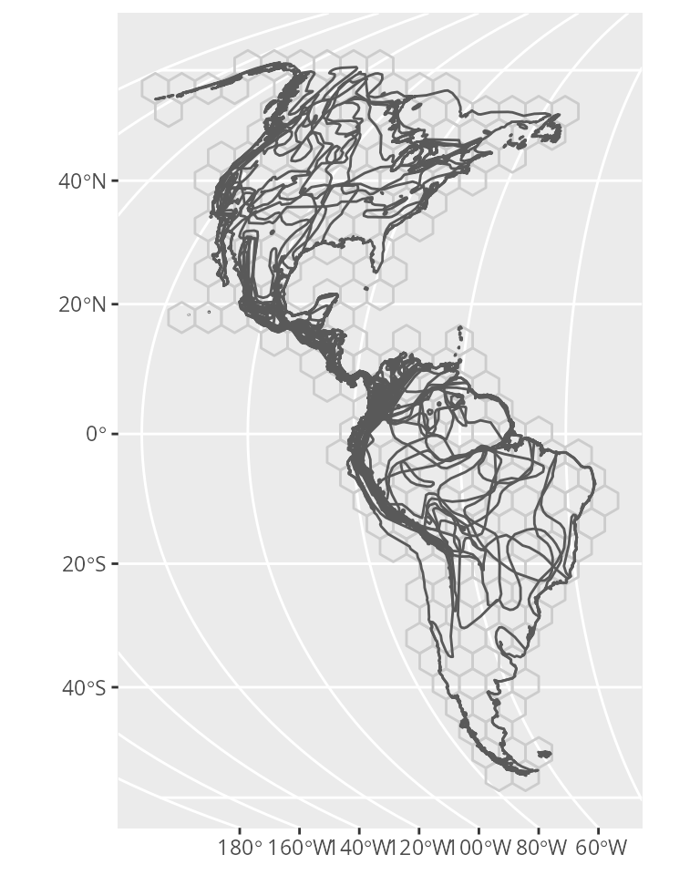
We’ll use the wrens dataset which is part of the package.
Raw data: wrens breeding range distribution and life history
head(wrens,3)
#> Simple feature collection with 3 features and 12 fields
#> geometry type:  MULTIPOLYGON
#> dimension:      XY
#> bbox:           xmin: -10184.52 ymin: 2019.465 xmax: -8391.563 ymax: 3447.125
#> CRS:            +proj=moll +lon_0=0 +x_0=0 +y_0=0 +datum=WGS84 +units=km +no_defs
#>   ID                    sci_name       com_name subspecies clutch_size
#> 1  1     Campylorhynchus_jocosus boucard's wren          1         3.5
#> 2  2     Campylorhynchus_gularis   spotted wren          1         4.0
#> 3  3 Campylorhynchus_yucatanicus   yucatan wren          1         3.0
#>   male_wing female_wing male_tarsus female_tarsus body_mass      data_src
#> 1     73.10       70.30        22.9          22.2      27.6 1,1,1,1,1,1,3
#> 2     74.00       71.75        24.0          24.0      30.1 1,2,1,1,1,1,3
#> 3     76.55       71.35        25.1          23.6      35.5 1,2,1,1,1,1,3
#>                         geometry breeding_range_area
#> 1 MULTIPOLYGON (((-9589.923 2...     68459.65 [km^2]
#> 2 MULTIPOLYGON (((-9469.687 2...    237890.51 [km^2]
#> 3 MULTIPOLYGON (((-8391.563 2...     11365.78 [km^2]
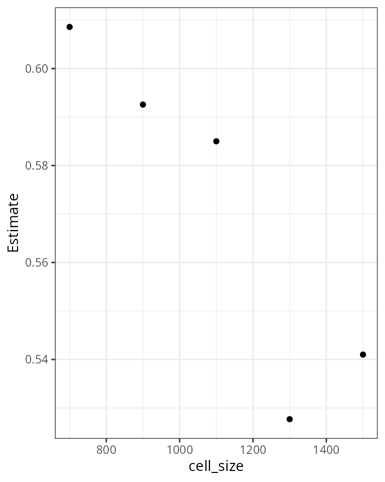
Case study 3: The influence of cell size on body size ~ species richness slope
1. assemblage level median body size ~ species richness slope for varying cell sizes.
cellSizes = seq(from = 700, to = 1500, length.out = 5)

FUN = function(g) {
  options(rmap.verbose = FALSE)

  con = rmap_connect()
  rmap_add_ranges(con, x = wrens, ID = 'sci_name')
  rmap_prepare(con, 'hex', cellsize=g)
  rmap_add_bio(con, wrens, 'sci_name')
  rmap_save_map(con)
  rmap_save_map(con, fun = 'median', src='wrens', v = 'male_tarsus', dst='median_male_tarsus')
  m = rmap_to_sf(con)

  # lm at assemblage level
  o = lm(scale(log(median_male_tarsus)) ~ sqrt(species_richness), m)  %>%
        summary %>% coefficients %>% data.frame %>% .[-1, ]

  o$cell_size = g

  options(rmap.verbose = TRUE)

  o

  }


o = lapply(cellSizes, FUN)   %>% rbindlist
2. Plot regression parameters for different cell sizes
Most of the variation here is due to spatial autocorrelation, a proper analysis requires a spatial model.